
In Depth Guide to Low Detection Limits
Why Low Detection Limits Matter in Trace Element Analysis
Low detection limits are the foundation of reliable trace element analysis — they define the smallest concentration of a substance that an analytical method can reliably distinguish from background noise.
Here is a quick-reference breakdown of the three core thresholds every lab professional needs to know:
| Term | What It Means | Typical Calculation |
|---|---|---|
| Limit of Blank (LOB) | Highest signal expected from a blank sample with no analyte present | Mean of blank + 1.645 × SD of blank |
| Limit of Detection (LOD) | Lowest concentration reliably distinguished from the blank | LOB + 1.645 × SD of low-concentration sample |
| Limit of Quantitation (LOQ) | Lowest concentration measurable with acceptable precision and accuracy | Approximately 10 × SD of blank |
These three thresholds are not interchangeable — and mixing them up leads to reporting errors, failed audits, and missed detections in critical samples.
For industries like aerospace, pharmaceuticals, and environmental testing, the stakes are high. A method that cannot detect a contaminant at the required concentration level is not just imprecise — it is unfit for purpose.
Modern techniques like ICP-MS can push detection limits into the picograms-per-liter (pg/L) range for many elements. But achieving those numbers in real samples — not just in pure water — requires a clear understanding of how detection limits are defined, calculated, and validated.
This guide covers everything: the statistics behind detection limits, the difference between instrument and method detection limits, how matrix effects raise your practical floor, and what regulatory bodies like IUPAC, the EPA, and CLSI actually require.
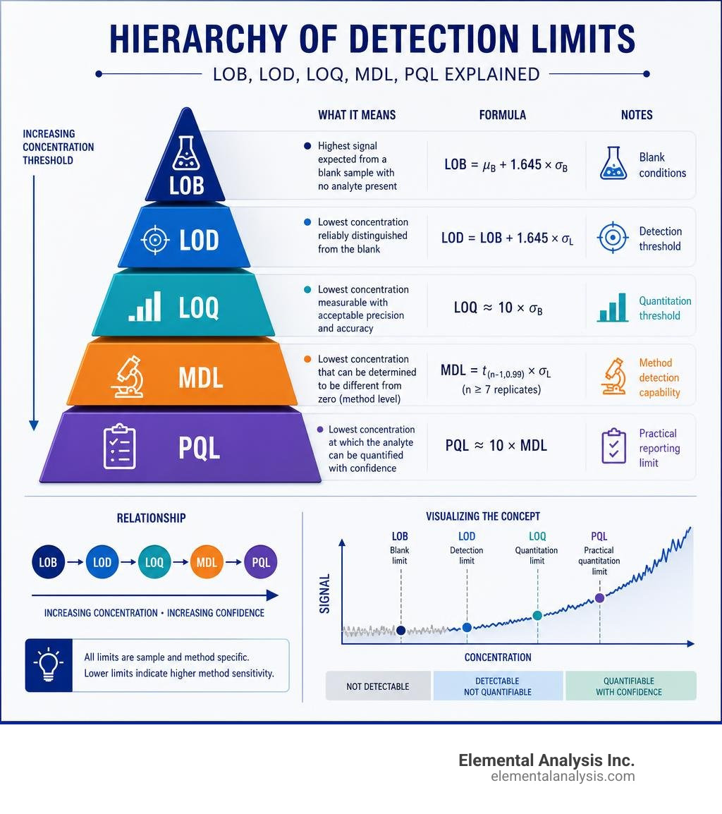
Defining the Thresholds: LOB, LOD, and LOQ
In trace analysis, knowing whether a target compound is present is rarely a simple “yes” or “no” question. As we push analytical instrumentation to its physical limits, we enter a statistical gray zone where the instrument’s detector registers a signal even when analyzing a completely blank sample. To make sense of this noise, we must establish clear, mathematically sound boundaries.
The Clinical and Laboratory Standards Institute (CLSI) EP17 guideline outlines a highly structured, three-tier hierarchy to define these boundaries, as detailed in the comprehensive overview on the Limit of Blank, Limit of Detection and Limit of Quantitation – PMC – NIH. These three parameters—Limit of Blank (LOB), Limit of Detection (LOD), and Limit of Quantitation (LOQ)—are the pillars of low-concentration measurement.
- Limit of Blank (LOB): This is the highest apparent analyte concentration we expect to see when testing replicates of a blank sample that contains absolutely no analyte. It represents the baseline noise of the system.
- Limit of Detection (LOD): This is the lowest concentration of an analyte that can be reliably distinguished from the LOB. It is the point at which we can confidently say, “The analyte is definitely present,” even if we cannot measure its exact concentration with high precision.
- Limit of Quantitation (LOQ): This is the lowest concentration at which the analyte can not only be detected but also quantified with a predefined level of precision and accuracy.
Understanding these differences is critical for real-world decision-making. For instance, in clinical assays like thyroid-stimulating hormone (TSH) testing, being able to distinguish euthyroid from hyperthyroid patients relies entirely on functional sensitivity at the extreme low end of the analytical range. If a laboratory confuses its LOD with its LOQ, it risks reporting quantitative values that are highly inaccurate, leading to incorrect diagnoses or regulatory compliance failures.
The Statistical Foundation of Low Detection Limits
Determining low detection limits is fundamentally an exercise in risk management. Whenever we make a measurement near the baseline noise of an instrument, we face two primary types of statistical errors:
- Type I Error (Alpha Error / False Positive): This occurs when we conclude that an analyte is present when it is actually absent. We mistake random instrument noise for a true analytical signal.
- Type II Error (Beta Error / False Negative): This occurs when we conclude that an analyte is absent when it is actually present. The true signal from the analyte is swallowed up by the baseline noise, and we miss it.
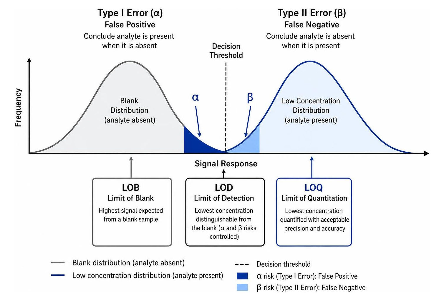
When establishing the LOB, we typically set the alpha ($\alpha$) error at 5% (or 0.05). Under a standard Gaussian (normal) distribution, this means that 95% of blank measurements will fall below the LOB, leaving a 5% chance that a true blank sample will yield a signal higher than the LOB and be flagged as a false positive.
The LOD is then calculated by shifting the distribution curve to the right, ensuring that a low-concentration sample has no more than a 5% beta ($\beta$) risk of falling below the LOB (yielding a false negative). This statistical balance is crucial. If we set our decision threshold too low, we flood our data with false positives; if we set it too high, we fail to detect trace contaminants that could pose severe environmental or health risks. For a deeper look into the mathematical handling of these statistical boundaries, researchers often consult Statistical methods for assays with limits of detection – PMC.
Mathematical Derivation and Calculation of LOD
To calculate these values in a routine laboratory setting, we rely on standard deviations of blanks or low-concentration spikes, standard confidence factors, and calibration curves.
Assuming a normal distribution of data points, the mathematical formulas are structured as follows:
$$\text{LOB} = \text{Mean}{\text{blank}} + 1.645 \times (\text{SD}{\text{blank}})$$
$$\text{LOD} = \text{LOB} + 1.645 \times (\text{SD}_{\text{low concentration sample}})$$
If the standard deviations of the blank and the low-concentration sample are roughly equal ($\sigma0 \approx \sigmaD$), these equations simplify to the classic IUPAC definition:
$$\text{LOD} \approx 3.29 \times \text{SD}_{\text{blank}}$$
In chromatographic methods, a common alternative is to calculate the LOD using the slope of the calibration curve ($a$) and the y-intercept standard deviation ($s_b$), as detailed by The Limit of Detection | LCGC International – Chromatography Online:
$$\text{LOD} = \frac{y + 3.2s – b}{a}$$
Where $y$ is the average blank signal, $s$ is the standard deviation, $b$ is the y-intercept, and $a$ is the slope of the linear calibration curve.
To obtain statistically rigorous standard deviations, we recommend analyzing a minimum of 7 to 10 independent blank or low-concentration replicate samples. Using fewer replicates reduces the degrees of freedom, requiring the use of Student’s t-values (such as $t = 3.14$ for 99% confidence with 7 samples) instead of the standard 1.645 or 3.0 multipliers, which ultimately raises your calculated detection limits.
Types of Low Detection Limits in Analytical Chemistry
In practical laboratory operations, “detection limit” is an umbrella term. Depending on where and how the measurement is made, we must distinguish between several types of limits.
| Limit Type | Definition | Key Factors Involved | Typical Use Case |
|---|---|---|---|
| Instrument Detection Limit (IDL) | The lowest concentration of analyte detectable by the instrument alone. | Pure solvent, minimal noise, optimized settings. | Instrument benchmarking and performance verification. |
| Method Detection Limit (MDL) | The lowest concentration detectable taking the entire preparation process into account. | Acid digestions, dilutions, reagent contaminants, filter blanks. | Regulatory compliance reporting for real-world samples. |
| Practical Quantitation Limit (PQL) | The lowest level that can be reliably achieved within specified limits of precision during routine laboratory operating conditions. | Matrix interferences, operator variability, long-term instrument drift. | Commercial reporting limits and industrial water monitoring. |
Instrument Detection Limit vs. Method Detection Limit
The gap between the Instrument Detection Limit (IDL) and the Method Detection Limit (MDL) is one of the most common sources of confusion in trace analysis.
The IDL is estimated using a clean, pure standards-in-solvent mixture under ideal conditions. It represents the absolute best-case scenario for the instrument’s hardware. However, real-world samples are rarely clean. They must be collected, transported, digested in strong acids, filtered, and diluted.
Every single step of sample preparation introduces two things: dilution and potential contamination. For example, if we digest 0.1 g of a soil sample and dilute it to a final volume of 10 mL, we have introduced a 100x dilution factor. If the instrument’s IDL for a heavy metal is 1 ppt (part-per-trillion), the theoretical best MDL we could achieve after accounting for dilution is 100 ppt—assuming zero contamination from our reagents or digestion vessels.
In reality, reagents, acids, and laboratory glassware contain trace impurities that add to the blank signal. Thus, the MDL is always higher than the IDL, sometimes by an order of magnitude or more. For a step-by-step breakdown of how sample preparation variables impact final results, see our ICP-MS Lab Guide: How to Get Accurate Trace Element Testing.
Practical Quantitation Limits and Reporting Limits
While the MDL tells us what we can detect with statistical confidence, the Practical Quantitation Limit (PQL) or Lower Reporting Limit (LRL) tells us what we can reliably report day in and day out with acceptable accuracy.
When reporting data to environmental databases or regulatory portals, we often encounter “censored data”—results that fall below the reporting limit (often recorded as “non-detects” or “< MDL"). Managing this censored data is highly regulated. For instance, when submitting water quality data to the EPA's Water Quality Exchange (WQX) schema or the Water Quality Portal (WQP), laboratories must follow strict rules.
Rather than entering a arbitrary “zero” or using special characters like “<" directly in the value field, standard practices require leaving the main result value blank and populating the "Result Detection Condition" (e.g., Not Detected or Below Reporting Limit) alongside the specific “Detection Limit Type”, “Value”, and “Unit”. This prevents data users from misinterpreting censored data during long-term statistical trends and environmental impact assessments.
Overcoming Matrix Effects and Interferences in Trace Analysis
The matrix is everything that is not the analyte of interest in your sample. In complex samples like soils, wastewater, biological tissues, or industrial chemicals, the matrix can severely disrupt our ability to achieve low detection limits.

These interferences generally fall into three categories:
- Spectral Interferences: Occur when an interfering species shares the same mass-to-charge ($m/z$) ratio or emission wavelength as the target analyte. A classic example in ICP-MS is the overlap of the argon chloride polyatomic ion ($^{40}\text{Ar}^{35}\text{Cl}^{+}$) with arsenic ($^{75}\text{As}$).
- Physical Interferences: Caused by differences in viscosity, surface tension, or density between the calibration standards and the actual sample matrix. High-salt matrices can clog nebulizers and alter sample uptake rates, suppressing the analytical signal.
- Chemical Interferences: Occur when chemical species in the sample matrix prevent the analyte from atomizing or ionizing efficiently in the plasma or flame.
To explore the physics of how these interferences occur inside a high-temperature plasma, read our detailed guide on The Ins and Outs of Inductively Coupled Plasma Mass Spectrometry.
Strategies for Achieving Low Detection Limits in ICP-MS
Achieving parts-per-trillion (ppt) or parts-per-quadrillion (ppq) detection limits outside of a cleanroom requires a combination of strict contamination control and advanced instrument engineering.
- Laminar Flow Environments: Preparing samples inside a Class 100 laminar flow box can reduce ambient particle concentrations by a factor of 10,000, preventing dust from contaminating ultra-trace samples.
- Sub-Boiling Acid Distillation: Commercial high-purity acids can still contain trace metal impurities. Using sub-boiling distillation in quartz or Teflon stills allows laboratories to produce ultra-pure acids with contaminant levels below 10 ppt.
- Collision-Reaction Cells (CRC): Modern ICP-MS instruments use helium collision gas (to filter out larger polyatomic interferences via kinetic energy discrimination) or reactive gases like hydrogen or oxygen to chemically destroy interferences. For example, using hydrogen reaction gas in “BOOST mode” (applying a positive bias voltage to the skimmer cone) can reduce the $^{40}\text{Ar}^{16}\text{O}^{+}$ interference on iron, achieving an ultra-low detection limit of 1.5 ng/L (ppt) for $^{56}\text{Fe}$.
- Single-Particle ICP-MS (spICP-MS): This cutting-edge technique allows us to count individual nanoparticles and measure their size distribution. While conventional ICP-MS has a detection floor around $10^6$ particles/mL, spICP-MS can detect down to 100 particles/mL by measuring rapid, individual ion bursts.
For a deeper dive into the inner workings of plasma-based mass spectrometers, see our article ICP-MS Explained: How We Weigh Atoms in a Plasma Fire.
Advanced Sensors and Nanomaterials for Ultra-Trace Detection
While plasma spectrometry remains the gold standard for metals, the push for low detection limits has driven incredible innovations in electrochemical and solid-state sensors for organic molecules and ions.
A prime example is the development of transconductance-enhanced graphene ion-sensitive field-effect transistors (ISFETs). By optimizing the thickness of the ion-sensitive membrane (ISM) to 3.6 $\mu\text{m}$ and maximizing the channel width-to-length ratio, researchers have achieved a record-low detection limit of 0.041 ppt ($4.8 \times 10^{-13}\text{ M}$) for nitrate ions, spanning nine orders of magnitude. The science behind this breakthrough is published in Ultra-sensitive nitrate-ion detection via transconductance-enhanced graphene ion-sensitive field-effect transistors | Microsystems & Nanoengineering.
Similarly, hybrid nanomaterials are revolutionizing food safety and environmental testing. An adsorption-enhanced electrochemical sensor combining CTAB-silica and APTES-functionalized multi-walled carbon nanotubes has been developed to detect Bisphenol A (BPA) at ultra-trace levels. This platform achieves a detection limit of $1.2 \times 10^{-9}\text{ M}$ ($S/N = 3$) across three distinct linear ranges, as detailed in the study Hybrid CTAB–Silica and APTES-Functionalized Multi-Walled Carbon Nanotubes for Adsorption-Enhanced Electrochemical Detection of Bisphenol A in Environmental and Food Samples – IOPscience.
Furthermore, post-polymerization modifications of poly(diphenylacetylene) with ionic liquids containing bis(trifluoromethylsulfonyl)imide ($\text{Tf}_2\text{N}^{-}$) anions have pushed detection limits for explosives like picric acid down to an astonishing 0.6 nM. This research can be explored further in Ultrahigh sensitivity and extremely low limit of detection of picric acid with ionic-liquid modified poly(diphenylacetylene) – Journal of Materials Chemistry A (RSC Publishing).
Regulatory Guidelines and Best Practices for Validation
Achieving a low detection limit in a research lab is one thing; proving that your method meets the rigorous standards of international regulatory bodies is quite another.
Depending on your industry, you must align your validation protocols with different frameworks:
- IUPAC (International Union of Pure and Applied Chemistry): Focuses on chemical terminology, recommending a 3-sigma approach for LOD and a 10-sigma approach for LOQ based on the standard deviation of the blank.
- US EPA (Environmental Protection Agency): Governs environmental testing. The EPA’s MDL procedure requires analyzing at least seven spiked samples and seven blank samples over multiple days to account for instrument drift and operator variability.
- CLSI (Clinical and Laboratory Standards Institute): Guidelines like EP17 are the gold standard for clinical diagnostics and medical devices, utilizing the LOB, LOD, and LOQ framework with strict requirements on sample size (often requiring 20 to 60 replicates across multiple instrument lots).
For a comprehensive look at how these regulations apply to toxicological screening, see our resource Heavy Metal Analysis by ICP-MS: The Ultimate Guide to Screening Toxins.
Harmonizing Standards Across IUPAC, EPA, and CLSI
While these organizations use slightly different terminologies and statistical multipliers, they all share a common goal: ensuring that analytical measurements are “fit for purpose.”
To maintain compliance across different frameworks, laboratories must document their standard operating procedures (SOPs) with extreme care. This includes establishing clear rules for when a method must be re-validated (such as after major instrument maintenance, a change in reagent lots, or moving to a new facility). For a broader discussion on the role of validation in trace testing, refer to ICP-MS Testing: Unleashing the Power of Plasma for Elemental Analysis.
Local regulatory context also plays a massive role. For example, municipal water authorities and industrial dischargers in Kentucky must ensure their testing methods align with state-specific enforcement standards, such as those maintained by the Kentucky Energy and Environment Cabinet.
Protocol for Validating and Reporting Trace Measurements
To validate and report trace and ultra-trace measurements with absolute confidence, we recommend following this systematic protocol:
- Run Blank Replicates: Analyze a minimum of 10 independent preparation blanks using the exact reagents and labware that will be used for real samples.
- Calculate LOB: Determine the mean and standard deviation of these blanks to establish your LOB.
- Spike at Low Concentrations: Spike a clean matrix with your target analytes at a concentration 2 to 5 times your estimated LOB. Analyze at least 7 to 10 replicates of this spiked sample.
- Calculate LOD and LOQ: Use the standard deviation of these low-concentration replicates to calculate your LOD and LOQ.
- Verify the LOD: Analyze a sample spiked exactly at your calculated LOD. Ensure that no more than 5% of these measurements fall below your LOB threshold (verifying a low false-negative rate).
- Report Transparently: When reporting results near the detection limits, always specify the exact method used to calculate the limits, the sample preparation steps (including dilution factors), and provide the raw standard deviation data.
Frequently Asked Questions About Detection Limits
What is the difference between LOD and LOQ?
The LOD (Limit of Detection) is the lowest concentration of an analyte that can be reliably detected (distinguished from the blank) with statistical confidence, but not necessarily quantified with high precision. The LOQ (Limit of Quantitation) is the lowest concentration that can be quantified with an acceptable level of precision (repeatability) and accuracy (bias), typically defined as 10 times the standard deviation of the blank.
Why are method detection limits always higher than instrument detection limits?
Method detection limits (MDLs) account for the entire analytical process, including sample collection, acid digestion, filtration, and dilution, all of which dilute the sample and introduce trace contaminants from reagents and laboratory equipment. Instrument detection limits (IDLs) are measured using pure, uncontaminated standards injected directly into the instrument under perfect, optimized conditions.
How do matrix interferences affect the limit of detection?
Matrix interferences can suppress or enhance the analytical signal, overlap with the analyte’s signal (spectral interference), or increase the baseline noise of the instrument. Because detection limits are mathematically tied to the standard deviation of the background noise, any increase in background noise or reduction in signal intensity directly raises (worsens) the detection limit.
Conclusion
Understanding and achieving low detection limits is not just about having the most sensitive instrument on the market—it is about mastering the entire analytical ecosystem. From the statistical risk of false positives to the meticulous chemistry of sample preparation and contamination control, every step of the process dictates the reliability of your trace-level data.
At Elemental Analysis Inc., we specialize in trace element identification, quantification, and speciation services across a wide range of industries. As the first commercial Proton Induced X-ray Emission (PIXE) laboratory, we offer a unique blend of non-destructive and destructive testing techniques, delivering rapid turnaround times and competitive pricing. Whether you are analyzing high-purity materials, environmental water samples, or complex geological matrices, our team in Lexington, Kentucky, is dedicated to helping you achieve the highest levels of analytical accuracy.
To learn more about our trace analysis capabilities and how we can support your testing needs, visit our Elemental Analysis Inc. Services page today.