A Simple Guide to ICP AES and OES Analysis

What Is ICP AES Analysis and How Does It Work?

ICP AES analysis (Inductively Coupled Plasma Atomic Emission Spectroscopy)—often called ICP-OES—is a fast, multi-element testing technique used to identify and measure metals and metalloids in liquid and solid samples.

Here is how the process works in three simple steps:

1. Aerosolization: A liquid sample is pumped into a nebulizer, which turns it into a fine mist.
2. Plasma Excitation: The mist enters an argon plasma torch heated to roughly 6,000–10,000 K. The extreme heat vaporizes the sample, breaks it down into individual atoms, and excites its electrons.
3. Optical Measurement: As electrons fall back to their ground energy state, they release photons of light at characteristic wavelengths. A spectrometer measures these light wavelengths to identify which elements are present, while the light intensity reveals their exact concentration.

Think of it like holding a copper wire in a candle flame and watching it glow bright green. Every element has its own distinct color signature.

Modern ICP-AES systems measure light signals for over 40 elements simultaneously in less than two minutes. For lab managers and quality teams in aerospace, pharma, and environmental testing, it delivers rapid turnaround, broad linear dynamic ranges, and parts-per-billion (ppb) detection limits across complex sample matrices.

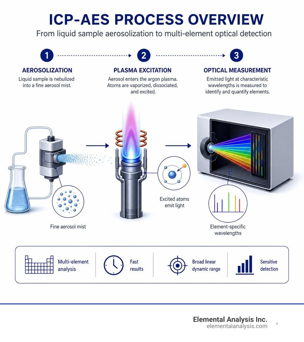
ICP AES analysis terms simplified:

• ICP MS elemental analysis
• trace impurities analysis
• elemental impurities testing

Understanding the Fundamentals of ICP AES Analysis

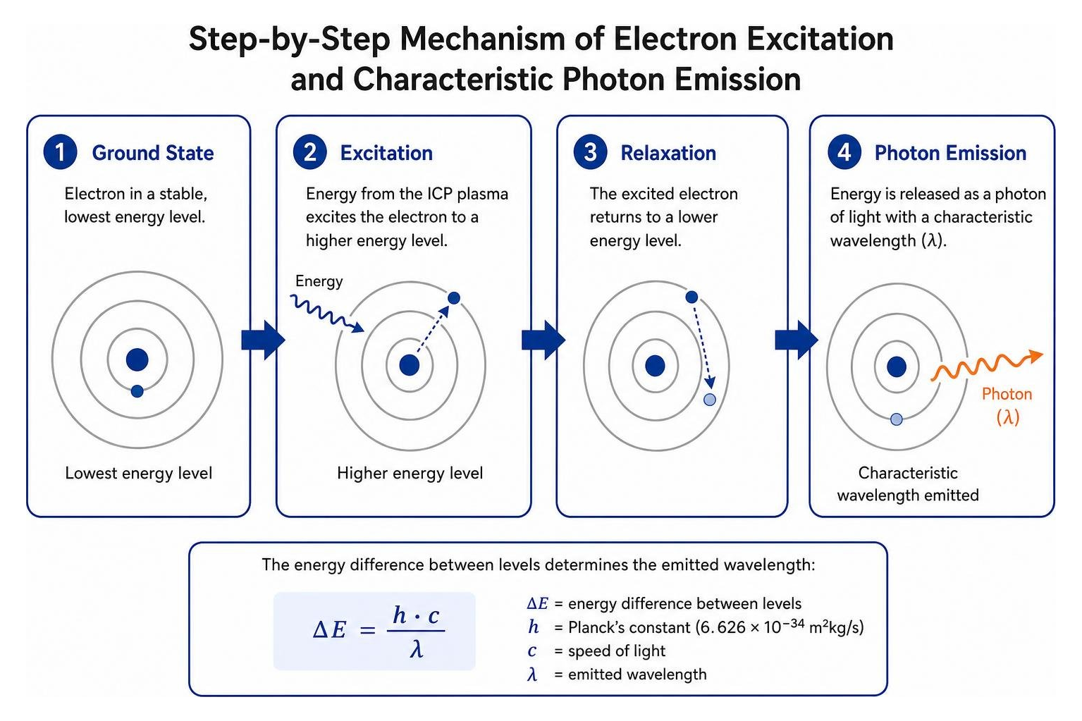
At its core, optical emission spectrometry relies on the predictable physics of electron excitation. When energy is introduced into an atom, its electrons absorb that energy and jump from their stable ground states to higher, unstable electronic orbitals. As these excited electrons drop back down to lower energy configurations, they release the excess energy as electromagnetic radiation—photons of light.

The energy difference between these quantum energy levels ($\Delta E$) determines the specific wavelength ($\lambda$) of the emitted photon according to Planck’s equation:

$$\Delta E = \frac{h \cdot c}{\lambda}$$

Where:

• $h$ is Planck’s constant ($6.626 \times 10^{-34} \text{ m}^2\text{kg/s}$)
• $c$ is the speed of light
• $\lambda$ is the emitted wavelength

Because every element on the periodic table possesses a unique electronic shell configuration, each element emits a distinct pattern of spectral lines.

To initiate this process reliably across dozens of elements simultaneously, we use a radio-frequency (RF) induced argon plasma. The RF generator delivers typically 1.0 to 1.5 kW of forward power into an induction coil wrapped around a quartz torch. An initial spark ionizes argon gas flowing through the torch, stripping electrons that accelerate within the oscillating magnetic field. Collisions between accelerated electrons and neutral argon atoms generate a self-sustaining, torch-shaped plasma reaching core temperatures up to 10,000 K.

For a deeper dive into the hardware and physical mechanisms sustaining these extreme states of matter, explore An Essential Guide to Inductively Coupled Plasma.

How ICP-AES and ICP-OES Systems Generate Atomic Spectra

Converting a bottled liquid sample into discrete atomic photon emissions requires a finely balanced sample introduction train:

1. Peristaltic Pumping & Nebulization: A peristaltic pump delivers the liquid at a continuous flow rate (typically 1 to 2 mL/min) into a concentric or cross-flow nebulizer. High-velocity argon gas sheers the liquid stream into a fine aerosol droplet suspension.
2. Spray Chamber Fractionation: The aerosol travels through a cyclonic or Scott double-pass spray chamber. Only droplets smaller than approximately 5 to 10 µm in diameter pass through to the injector tube; roughly 95% to 99% of the aspirated liquid mass drains out as waste.
3. Toroid Zone Desolvation & Atomization: The fine mist enters the central channel of the argon plasma torch (the toroid zone). Water or acid solvent instantly evaporates (desolvation), solid salts vaporize into gas phase molecules, and the extreme thermal energy dissociates molecules into free, uncharged atoms and ions (atomization and ionization).
4. Collision Excitation: Intense thermal collisions with energetic argon species pop electrons into excited states.
5. Dispersion & Detection: Light emitted as electrons relax travels into an optical spectrometer. A diffraction grating disperses the polychromatic light into discrete spectral wavelengths, focusing them onto high-sensitivity solid-state detectors such as Charge-Coupled Devices (CCD) or Charge-Injection Devices (CID).

Understanding how the argon torch vaporizes complex materials is central to modern spectroscopy, a topic explored further in Hot Stuff: How Inductively Coupled Argon Plasma Spectrometry Powers Modern Mass Spec.

Axial vs. Radial Plasma Viewing Configurations

Modern spectrometers use one of two viewing orientations—or combine both in dual-view optics—to direct plasma light into the spectrometer:

• Axial Viewing: The spectrometer looks directly down the longitudinal axis of the plasma torch. Viewing along the full length of the central emission channel collects significantly more photons. This yields higher signal intensity and improves detection limits by a factor of 3 to 10 for clean matrices, making it ideal for low-concentration trace element determination.
• Radial Viewing: The spectrometer views the plasma side-on, perpendicular to the torch axis. By focusing only on the optimal normal analytical zone and avoiding the cooler plasma tail, radial viewing reduces matrix interferences, handles high total dissolved solids (TDS > 1500 mg/L), and provides superior linearity at high analyte concentrations.

Parameter	Axial Plasma Viewing	Radial Plasma Viewing
Optical Alignment	Longitudinal down torch axis	Perpendicular side-on
Relative Sensitivity	High (3–10× lower detection limits)	Moderate
Background Intensity	Higher spectral background	Lower spectral background
Matrix Interference	More susceptible to matrix shifts	Highly resistant to complex matrices
TDS Tolerance	Lower (< 0.2% typical)	High (up to 10–20% with appropriate hardware)
Optimal Use Case	Trace & ultra-trace environmental waters	High-salt brines, alloys, slurries, digests

According to horizontal testing standard frameworks such as Document CEN/TC/230/WG1/TG 12 N 5, selecting between axial and radial views allows labs to balance detection limits against physical matrix interferences when characterizing environmental wastes, industrial sludges, and digestates.

Sample Preparation and Digestion Protocols

A spectrometer can only measure what successfully enters its plasma torch as a homogeneous solution. Sample preparation is therefore the foundation of analytical accuracy. Choosing the correct digestion chemistry ensures that all target analytes dissolve into ionic form without volatilizing or precipitating during storage.

For a complete breakdown of preparatory workflows across analytical chemistry, check out A Quick Start Guide to Elemental Analysis Methods.

Acid Digestion and Lithium Metaborate Flux Fusion

The primary method for preparing solid inorganic samples is wet chemical acid digestion:

• Closed-Vessel Microwave Digestion: High-purity concentrated nitric acid ($\text{HNO}_3$, ~65–70%) breaks down organic structures and solubilizes most metals. Hydrochloric acid ($\text{HCl}$) is added to stabilize volatile or hydrolyzable elements like tin ($\text{Sn}$), antimony ($\text{Sb}$), molybdenum ($\text{Mo}$), and silver ($\text{Ag}$).
• Hydrofluoric Acid ($\text{HF}$) Additions: When dissolving silicate minerals, sands, or ceramics, HF is required to cleave strong silicon-oxygen bonds. However, HF volatilizes silicon as gaseous silicon tetrafluoride ($\text{SiF}_4$), preventing total silicon quantification.

For difficult geological matrices, rock cores, refractory minerals (containing titanium, chromium, and zirconium), and sediments, Lithium Metaborate ($\text{LiBO}_2$) Flux Fusion provides an alternative to multi-acid dissolution.

As outlined in ANALYSIS OF MAJOR AND TRACE ELEMENTS IN ROCKS, SEDIMENTS, AND INTERSTITIAL WATERS BY INDUCTIVELY COUPLED PLASMA-ATOMIC EMISSION SPECTROMETRY (ICP-AES), powdered geological samples are mixed in a 1:4 ratio with ultrapure $\text{LiBO}_2$ flux and a trace $\text{LiBr}$ wetting agent in a platinum-gold crucible. Heating to 1050 °C for 10–12 minutes produces a molten glass bead that dissolves completely in dilute nitric acid upon cooling. This completely dissolves resistant minerals while retaining all silica in solution without requiring hazardous HF additions.

Preparing Nanomaterials for ICP AES Analysis

Nanoparticles present specific preparation challenges. Protective organic surface capping agents (e.g., oleic acid, PEG, citrate) and low-vapor-pressure organic carrying solvents interfere with regular plasma nebulization, producing irregular carbon soot and matrix suppression.

To prepare nanomaterials:

1. Solvent Evaporation: Gently evaporate volatile organic solvents using low heat on an open block.
2. Organic Ligand Stripping: Treat residue with oxidizing agents (such as chloric acid or hot concentrated $\text{HNO}_3$) to fully decompose protective surfactant chains.
3. Complete Matrix Digestion: Digest remaining metallic cores using concentrated trace-metal grade acids until no particulate matter remains. Incomplete digestion prevents uniform droplet vaporization and artificially lowers concentration readings.
4. Nanopure Dilution: Dilute exclusively using ultrapure Type 1 water (resistivity $\ge 18.2 \text{ M}\Omega\cdot\text{cm}$). Standard tap or deionized water contains background trace iron and zinc that skew trace-level measurements.

Quantitative Calculations and Multiline Spectral Calibration

To convert raw photon emission counts into concentration values (e.g., mg/L or ppm), we construct a multi-point calibration curve using matrix-matched certified standard solutions.

Standard curves typically use a linear model:

$$I = m \cdot C + I_0$$

Where:

• $I$ is the measured net optical emission intensity
• $m$ is the calibration slope (sensitivity)
• $C$ is the analyte concentration
• $I_0$ is the background intensity of the calibration blank

To maintain measurement accuracy across broad dynamic ranges, regulatory protocols require calibration correlation coefficients ($r$) of at least 0.995, with Initial Calibration Verification (ICV) standards recovering within 90% to 110% of their certified values.

To understand how internal calibration standards normalize sample transport variations across complex runs, see Unlocking the Elements with ICP Laboratory Analysis.

Calculating Analyte Concentration, Stoichiometry, and Nanoparticle Surface Area in ICP AES Analysis

Once we determine the dissolved analyte concentration from the calibration curve, we can account for dilution factors, determine metal stoichiometry in bimetallic catalysts, and calculate physical properties like nanoparticle counts and surface area.

1. Calculating Original Solution Concentration

To calculate analyte concentration in the original sample before dilution:

$$C_{\text{original}} (\text{mg/L}) = C_{\text{measured}} \times \left( \frac{V_{\text{final}}}{V_{\text{aliquot}}} \right)$$

2. Determining Stoichiometric Ratios in Bimetallic Nanoparticles

For synthesized multi-metal alloys (such as Fe-Cu nanocrystals):

• Measure the mass concentration ($C$, in mg/L) of Metal A ($\text{Fe}$) and Metal B ($\text{Cu}$).
• Convert mass concentrations to molar concentrations:

$$M_{\text{Fe}} = \frac{C_{\text{Fe}}}{MW_{\text{Fe}}}, \quad M_{\text{Cu}} = \frac{C_{\text{Cu}}}{MW_{\text{Cu}}}$$

• Calculate the molar ratio:

$$\text{Stoichiometric Ratio} = \frac{M_{\text{Fe}}}{M_{\text{Cu}}}$$

This confirms whether synthetic chemical additions match actual crystal incorporation.

3. Calculating Nanoparticle Particle Counts and Combined Surface Area

With known core geometry (e.g., spherical particles with diameter $d = 7\text{ nm}$) and crystallographic density, elemental data can be converted into physical metrics:

• Mass per Particle: Volume of a 7 nm sphere: $$V_p = \frac{4}{3}\pi r^3 = \frac{4}{3}\pi (3.5 \times 10^{-7}\text{ cm})^3 \approx 1.796 \times 10^{-19}\text{ cm}^3$$ For magnetite ($\text{Fe}3\text{O}4$, density $\rho = 5.18\text{ g/cm}^3$), mass per particle is: $$mp = \rho \cdot Vp \approx 9.30 \times 10^{-19}\text{ g}$$
• Iron Content per Particle: $\text{Fe}_3\text{O}_4$ is ~72.36% Fe by mass, meaning one particle contains $\approx 6.73 \times 10^{-19}\text{ g Fe}$.
• Particle Concentration: In a solution containing 51,040 mg/L (51.04 g/L) Fe:

$$\text{Particles/L} = \frac{51.04\text{ g Fe/L}}{6.73 \times 10^{-19}\text{ g Fe/particle}} \approx 5.5 \times 10^{19}\text{ particles/L}$$

• Combined Surface Area: The surface area of one 7 nm sphere is $A_p = 4\pi r^2 \approx 1.539 \times 10^{-16}\text{ m}^2$. Multiplying by total particles:

$$\text{Total Area} = (5.5 \times 10^{19}\text{ particles}) \times (1.539 \times 10^{-16}\text{ m}^2) \approx 8,465\text{ m}^2\text{/L}$$

One single liter of this iron nanoparticle solution contains over $8,400\text{ m}^2$ of active surface area—equivalent to roughly 1.5 American football fields.

Multiline Analysis and Inter-Element Spectral Interference Mitigation

Spectral interferences occur when light emitted by concomitant elements in the sample overlaps with the target analyte’s primary analytical wavelength (e.g., Fe at 238.204 nm overlapping with Co at 238.892 nm). In complex matrices like structural steel, thousands of overlapping transition metal emission lines can lead to analytical bias if only a single wavelength is monitored.

Modern CCD and CID detectors capture full spectra across 50,000+ identified emission lines simultaneously, enabling multiline analysis:

1. Multi-Wavelength Acquisition: Rather than relying on a single emission line, the instrument captures two to five distinct wavelengths for each element.
2. Cross-Validation: Software models expected peak profiles and synthetic spectra using pre-compiled reference libraries.
3. ANOVA Outlier Rejection: Discrepancies between individual line concentrations are evaluated using analysis-of-variance (ANOVA) statistics. If an unanticipated element (such as $120\text{ mg/L}$ tungsten interfering with copper at 217.895 nm) skews one emission line, the algorithm flags and eliminates that outlier line.

As detailed in research published by NIPPON, multiline analysis and automated matrix-matching systems provide accurate steel characterization in under 60 seconds, eliminating manual dissolution artifacts and rejecting unexpected spectral overlaps.

Standard Procedures for Airborne Particulates and Environmental Testing

Environmental and industrial hygiene laboratories routinely rely on ICP-AES to screen for airborne toxic dusts, hazardous soils, wastewater effluents, and workplace exposures.

Air Quality and Metal Particulate Monitoring via ASTM D7035

Airborne particulate sampling evaluates toxic workplace exposure to dusts and metal fumes (such as cadmium, chromium, lead, and manganese). Following standard industrial hygiene procedures:

• Personal air sampling pumps draw air through 37-mm Mixed Cellulose Ester (MCE) or PVC filter cassettes at a calibrated flow rate of $2.0\text{ L/min}$.
• Samples are digested using hot-plate acid mixtures of nitric acid ($\text{HNO}_3$), sulfuric acid ($\text{H}_2\text{SO}_4$), and hydrogen peroxide ($\text{H}_2\text{O}_2$) until organic matrix filter fibers are destroyed and SO3 white fumes evolve.
• The standardized protocol defined in METAL AND METALLOID PARTICULATES IN WORKPLACE ATMOSPHERES (ICP ANALYSIS) (OSHA Method ID-125G) demonstrates analytical error within $\pm25\%$ at a 95% confidence limit across 13 target elements, with detection limits reaching $0.0052\text{ }\mu\text{g}$ per sample for beryllium ($\text{Be}$) and $0.053\text{ }\mu\text{g}$ for cadmium ($\text{Cd}$).

The overarching method scope is formalized under D7035 Standard Test Method for Determination of Metals and Metalloids in Airborne Particulate Matter by Inductively Coupled Plasma Atomic Emission Spectrometry (ICP-AES), which specifies procedures for measuring over 40 metals and metalloids in workplace air across soluble and total particulate fractions.

EPA Quality Assurance Protocols and Detection Limits

For hazardous waste, Superfund sites, and wastewater monitoring, laboratories adhere to EPA Contract Laboratory Program (CLP) specifications, such as EPA CONTRACT LABORATORY PROGRAM STATEMENT OF WORK FOR SUPERFUND ANALYTICAL METHODS Multi-Media, Multi-Concentration SFAM01.0 January 2019 – Exhibit D: Inorganic Methods.

Quality assurance protocols require:

• Instrument Detection Limit (IDL): Established by analyzing a minimum of 7 to 8 replicate blank spikes on consecutive days ($3 \times S_r$).
• Continuing Calibration Blanks & Verifications (CCB/CCV): Analyzed every 10 analytical samples to verify instrument stability within $\pm10\%$ recovery.
• Matrix Spikes (MS): Target recoveries must stay within 75% to 125% to confirm that dissolved salts do not cause physical or chemical suppression.

When choosing between screening tools for environmental pollutants, compare performance criteria using our guide on ICP Analysis for Heavy Metals: Choosing Between ICP-OES and ICP-MS.

Frequently Asked Questions About ICP-AES

What is the difference between ICP-AES and ICP-OES?

There is no functional difference between the two terms; they describe the exact same analytical technique.

• ICP-AES stands for Inductively Coupled Plasma Atomic Emission Spectroscopy.
• ICP-OES stands for Inductively Coupled Plasma Optical Emission Spectroscopy.

“Atomic” highlights the atomic excitation mechanism, while “Optical” highlights the light collection region (ultraviolet and visible spectrum, roughly 165–800 nm). Today, instrument manufacturers and standards organizations use the two terms interchangeably.

When should a lab choose ICP-AES over ICP-MS?

While Inductively Coupled Plasma Mass Spectrometry (ICP-MS) delivers lower detection limits (parts-per-trillion vs. parts-per-billion), ICP-AES remains the preferred choice when:

• High Total Dissolved Solids (TDS): Samples contain heavy salt, soil, or acid matrices (> 0.2% up to 10–20% TDS) that would clog an ICP-MS interface cone orifice.
• Major and Minor Element Quantification: Elements are present in high concentrations (ppm to weight-percent levels), where ICP-MS detectors would saturate without substantial dilution.
• Cost Efficiency & Throughput: ICP-AES systems have lower argon consumption, simpler consumable requirements, and lower capital investment.

For an in-depth breakdown of mass spectrometry capabilities, read The Ultimate Guide to ICP Mass Spectrometry and Elemental Analysis.

How do you correct for spectral interferences in complex metal matrices?

Analytical chemists apply several strategies to prevent spectral overlap from compromising sample data:

1. Alternate Line Selection: Choose secondary or tertiary emission lines separated by at least 15 nm from known matrix lines.
2. Background Correction: Set off-peak background subtraction points on one or both sides of the analyte peak where the baseline is flat and free of interferents.
3. Inter-Element Correction (IEC) Equations: Measure standard solutions of the interfering element alone, determine the ratio of false signal produced at the analyte line, and subtract that value dynamically during analysis.
4. Internal Standardization: Add non-interfering internal standards (such as Yttrium or Scandium) to correct for physical viscosity and nebulization differences between standards and samples.

Conclusion

ICP-AES remains a core analytical technique in modern elemental chemistry. By pairing the extreme temperatures of RF argon plasma with high-resolution solid-state optical spectrometers, it delivers fast, multi-element quantification across diverse matrices—from alloy steels and nanoparticles to environmental waters and workplace air filters.

At Elemental Analysis Inc., located in Lexington KY, Kentucky USA, we specialize in high-precision inorganic and elemental characterization. Our team combines spectroscopy with complementary techniques—including PIXE, ICP-MS, and automated combustion methods—to provide rapid turnarounds, regulatory-grade quality control, and testing for materials across industries.

To discuss your testing requirements or request a custom analysis, visit our ICP testing and spectroscopic analysis service center.