Inside the Fiery World of Inductively Coupled Plasma Emission

Understanding Inductively Coupled Plasma Emission and How It Works

Inductively coupled plasma emission is a high-precision analytical technique that uses an ultra-hot argon plasma to measure the elemental composition of a sample. By heating liquid aerosols to temperatures between 5,000 K and 10,000 K, the plasma instantly vaporizes, atomizes, and excites the sample. As these excited atoms and ions return to lower energy states, they emit light at specific, element-identifying wavelengths.

By measuring the exact wavelength and intensity of that emitted light, an optical spectrometer can identify and quantify over 70 elements at once—from major percentage levels down to trace parts-per-billion (ppb) concentrations.

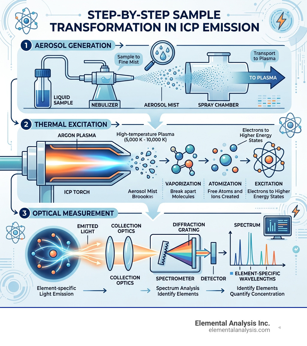
Here is the three-step breakdown of how the process works in real time:

1. Aerosol Generation: A nebulizer turns your liquid sample into a fine mist, carrying roughly 2% to 3% of the finest droplets into the center of the plasma torch.
2. Thermal Excitation: The radio-frequency-sustained argon plasma rips the aerosol droplets apart, converting molecules into free, excited atoms and ions.
3. Optical Measurement: High-resolution spectrometers capture the element-specific light emission, comparing the signal intensity against calibration standards to deliver fast, quantitative results.

Whether you are qualifying aerospace alloys, testing pharmaceutical raw materials, or monitoring environmental wastewater, this technique gives you rapid, multi-element data with exceptional matrix tolerance.

Basic inductively coupled plasma emission vocab:

• inductively coupled plasma
• induced coupled plasma
• inductively coupled argon plasma spectrometry

Fundamentals of Inductively Coupled Plasma Emission and Plasma Generation

Generating an analytical plasma torch requires a balance of electromagnetic physics, radio-frequency (RF) power, and precise gas dynamics. Modern spectrometers rely on an RF generator operating at standard industrial frequencies, typically 27.12 MHz or 40.68 MHz (within the broader 27–41 MHz range), delivering between 1250 and 1550 W of power into an induction coil.

To create the plasma, high-purity argon gas is pumped through the torch assembly at a total consumption rate of around 18 L/min. When the RF coil is energized, it creates a fluctuating magnetic field. A high-voltage Tesla spark seeds initial “seed electrons” into the argon stream. As dictated by the Faraday-Lenz law of electromagnetic induction, the time-varying magnetic field induces an electric field that forces electrons into circular, closed paths within the quartz torch.

These accelerated electrons collide with neutral argon atoms, knocking off secondary electrons in an avalanche ionization process. Once sustained, the system enters the inductive mode (H-mode), establishing a stable, high-density discharge with an electron density on the order of $10^{15}\text{ cm}^{-3}$. To dive deeper into the physical chemistry underlying these high-temperature discharges, explore our guide to inductively coupled plasma and review classic inductively coupled plasma principles.

Plasma Torch Mechanics and Temperature Zones

The plasma torch itself consists of three concentric quartz tubes: the outer tube, the intermediate tube, and the central injector tube. Each channel has a distinct operational role:

• Outer Tube (Coolant/Plasma Gas): Introduces argon tangentially at 12–18 L/min. This high-velocity vortex thermalizes the plasma and keeps the 5,000–10,000 K core from melting the quartz walls.
• Intermediate Tube (Auxiliary Gas): Delivers argon at 0.5–1.5 L/min to position the base of the plasma above the injector tip, preventing thermal erosion.
• Center Injector Tube (Nebulizer/Carrier Gas): Uses a narrow bore (typically 1.5–2.5 mm ID) to punch a cool central channel through the toroidal plasma at 0.6–1.0 L/min, transporting sample aerosols directly through the core.

Because the induction coil transfers energy primarily to the outer perimeter, the plasma forms a donut-like (toroidal) geometry. The hottest outer regions reach 9,000–10,000 K, while the central analytical channel through which the sample passes sits between 5,500 K and 6,500 K—comparable to the temperature of the Sun’s photosphere. Under these extreme thermal conditions, the degree of ionization exceeds 90% for roughly 60 elements on the periodic table.

Sample Aerosolization and Inductively Coupled Plasma Emission Mechanics

Before any light emission occurs, a peristaltic pump draws liquid sample into a nebulizer, mixing it with pressurized argon to form a cloud of fine droplets. This aerosol enters a spray chamber designed to remove large droplets. Only the finest mist—roughly 2% to 3% of the total sample volume—has low enough inertia to navigate the chamber baffling and travel into the central injector.

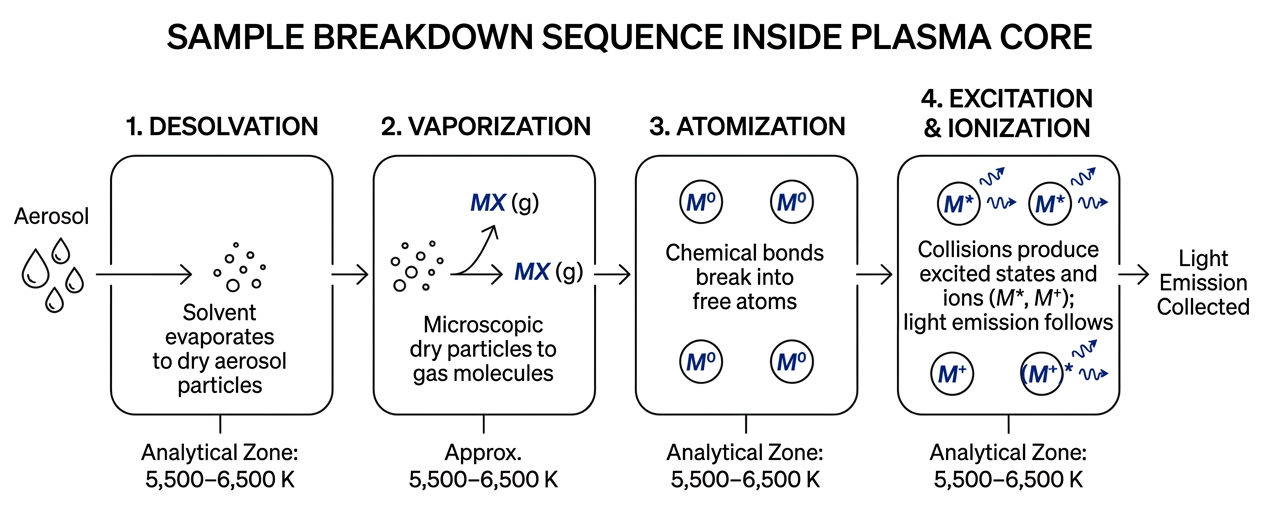
Once inside the torch’s analytical channel, the sample undergoes an ultra-fast sequence of physical and chemical transformations:

1. Desolvation: Solvent evaporates instantly, leaving microscopic dry aerosol salt particles.
2. Vaporization & Atomization: High temperatures break chemical bonds, turning solid particles into gaseous molecules and then free ground-state atoms ($M^0$).
3. Excitation & Ionization: Collisions with energetic electrons and argon ions promote atoms to excited states ($M^$) or remove electrons entirely to form ground-state and excited ions ($M^+$, $(M^+)^$).
4. Thermal Light Emission: Within nanoseconds, excited atoms and ions relax back to lower energy ground states, releasing photons with discrete wavelengths corresponding to elemental energy differences ($\Delta E = h\nu = hc/\lambda$).

By mastering these mechanics, laboratories can track emission lines across broad concentration ranges. For an in-depth breakdown of these excitation dynamics, consult our article on understanding ICP chemistry.

Sample Introduction and Plasma Torch Viewing Configurations

Achieving low detection limits depends on how sample aerosols enter the torch and how the optical spectrometer views the resulting photon discharge.

Choosing the correct combination of nebulizer geometry, spray chamber design, and torch orientation allows analysts to tailor the instrument for clean drinking waters, heavy organic matrices, or high-salt slurries. Learn more about matching these configurations in our guide to ICP-AES and OES analysis.

Nebulizer Technologies and Solid Sampling

Different sample types require specialized introduction hardware to ensure steady aerosol generation and avoid physical clogging:

• Concentric Pneumatic Nebulizers: Glass or polymer units where argon gas surrounds a central capillary. They produce very fine aerosols for clean aqueous samples but are susceptible to particulate clogging.
• Cross-Flow Nebulizers: Argon and liquid streams meet at right angles through robust sapphire or gemstone orifices, providing greater tolerance for samples containing moderate suspended solids.
• Babington and V-Groove Nebulizers: Liquid flows down an open, grooved channel over a gas orifice. Because sample liquid is not forced through a narrow internal constriction, these systems handle high total dissolved solids (TDS), including seawater and mining brines, without clogging.
• Ultrasonic Nebulizers (USN): Liquid is pumped onto a vibrating piezoelectric transducer operating at megahertz frequencies. A built-in heating and desolvation condenser boosts aerosol transport efficiency from 2–3% up to 10–20%, lowering detection limits by a factor of 5 to 50 for clean matrices.
• Hydride Generation (HG): Reacts acidified liquid samples with sodium borohydride ($\text{NaBH}_4$) to convert elements like As, Se, Sb, and Te into volatile gaseous hydrides ($\text{AsH}_3$, $\text{H}_2\text{Se}$), achieving nearly 100% transport efficiency.
• Laser Ablation (LA) and Slurry Introduction: For direct solid sampling, a pulsed UV laser can micro-mill solid surfaces, generating dry aerosol particles transported straight into the torch without wet chemical digestion. Alternatively, finely milled solid particulates ($<5\,\mu\text{m}$) can be suspended in a liquid matrix and aspirated directly as a slurry.

Axial vs. Radial Torch Viewing

Modern instruments observe the plasma flame using two primary optical orientations: radial (side-on) viewing and axial (end-on) viewing. Many advanced systems feature dual-viewing optics or a Dual Side-On Interface (DSOI) that can toggle between or combine both approaches.

Viewing Mode	Optical Alignment	Sensitivity & Detection Limits	Matrix Tolerance (TDS)	Primary Analytical Best Use
Axial (End-On)	Look straight down the analytical channel	2–10× lower detection limits due to extended optical path length	Lower ($\le 1\text{–}2\%\text{ TDS}$); higher matrix-induced background	Trace and ultra-trace metal analysis in clean water and environmental matrices
Radial (Side-On)	Looks across the plasma flame horizontally	Higher detection limits (less optical path depth)	High tolerance ($>10\text{–}20\%\text{ TDS}$); reduced spectral and physical interferences	Concentrated brine, metal alloys, geological digests, and petrochemicals
Dual View / DSOI	Software selects or mirrors both views	Optimized sensitivity across trace and major lines	Wide operational range via automated viewing mode switching	Mixed-concentration testing (e.g., trace Pb alongside major Ca/Na)

Axial viewing captures light across the entire length of the analytical channel, which increases the photon signal and yields a 2- to 10-fold improvement in detection limits compared to radial viewing. However, looking down the full axis also captures emission from cooler outer plume zones, increasing spectral background. Radial viewing bypasses cooler fringe zones, making it the preferred approach for high-salt solutions and complex matrices.

Optical System Designs and Interference Management

Once photons leave the plasma, the spectrometer must separate, disperse, and detect individual spectral lines without overlapping adjacent wavelengths.

Because a single complex matrix can emit thousands of distinct atomic lines, optical resolution and interference correction determine overall data accuracy.

Spectrometer Geometries: Paschen-Runge, Echelle, and Czerny-Turner

Instrument designers utilize three primary optical mounting layouts to isolate element wavelengths:

1. Echelle Polychromator: The industry workhorse for simultaneous multi-element spectrometers. Light reflects off a coarse, high-angle echelle diffraction grating to achieve high spectral order separation. A secondary prism or cross-disperser splits overlapping orders perpendicularly. This produces a compact two-dimensional spectrum focused onto a solid-state detector—such as a Charge-Coupled Device (CCD) or Charge-Injection Device (CID)—capturing the full 130–800 nm wavelength range in a single exposure.
2. Paschen-Runge Mount: Fixes an entry slit, concave grating, and multiple detectors along a single focal curve known as a Rowland circle. This design avoids moving parts, offering mechanical stability, high optical throughput, and low-stray-light detection in the deep vacuum UV (VUV) region (130–160 nm) for non-metals like sulfur, phosphorus, and halogens.
3. Czerny-Turner Monochromator: Uses two concave mirrors and a rotatable planar diffraction grating to scan sequentially across target wavelengths. While slower than simultaneous polychromators, Czerny-Turner systems allow flexible wavelength selection and high resolution for targeted single-element testing.

Correcting Interferences in Inductively Coupled Plasma Emission Spectroscopy

Analytical accuracy requires systematic identification and correction of four main interference types:

• Spectral Line Overlaps: Occur when an emission line from a matrix element (such as iron, nickel, or aluminum) falls directly over an analyte’s target wavelength. Analysts correct spectral overlaps by selecting alternate interference-free wavelengths, applying mathematical Interelement Correction (IEC) equations, or using multivariate deconvolution software.
• Physical Interferences: Differences in sample viscosity, surface tension, or density alter nebulizer uptake rates and droplet sizing. These effects are minimized using peristaltic pump control, matrix-matched calibration standards, or internal standards (such as Yttrium, Scandium, or Indium) spiked uniformly into all blanks, standards, and samples.
• Chemical Interferences: Caused by the formation of stable, non-dissociating compounds in low-temperature flames. In an analytical ICP, the 6,000–10,000 K operating temperature breaks virtually all chemical bonds, rendering chemical interferences negligible.
• Memory Carryover Effects: High-concentration analytes or sticky hydride elements can linger on spray chamber walls and injector tips. Extending post-sample rinse cycles with matrix blanks eliminates cross-sample contamination.

To maintain stable operation across complex matrices, laboratories monitor the magnesium emission intensity ratio: $\text{Mg II (280.2 nm)} / \text{Mg I (285.2 nm)}$. A robust, well-coupled plasma yields an $\text{Mg II}/\text{Mg I}$ ratio of 10 or higher. If the ratio drops below 8, the plasma is thermally overloaded and prone to matrix-induced suppression. Detailed QA/QC protocols for background correction point selection and matrix verification are documented under standard EPA Method 6010B guidelines.

Industrial Applications and Analytical Performance

Inductively coupled plasma emission spectrometry is widely used across commercial testing laboratories due to its wide linear dynamic range (spanning 5 to 6 orders of magnitude), rapid sample throughput, and matrix resilience.

When selecting between optical emission and mass spectrometry techniques for your analytical workload, refer to our guide on choosing between ICP-OES and ICP-MS.

Performance Strengths Across Diverse Sample Types

From municipal utilities to advanced manufacturing plants, this emission technique supports a range of industrial testing needs:

• Environmental Water and Soil Monitoring: Rapidly measures heavy metals (Pb, Cd, Cr, Cu, Zn, Ni) and major minerals (Ca, Mg, Na, K) in industrial wastewater discharges, drinking water supplies, and superfund soil digests down to low-ppb levels.
• Petrochemicals and Lubricating Oils: Diluting used lubricants in organic solvents (such as kerosene, xylene, or mineral spirits) allows direct measurement of wear metals (Fe, Cu, Al) and additive packages (Zn, P, Ca, Ba) to predict engine wear and schedule preventative maintenance.
• Geology, Mining, and Metallurgy: High-temperature plasma ionization breaks down refractory oxides (such as zirconium, tantalum, and tungsten), making it an effective choice for mining exploration, grade assays, and alloy verification without requiring volatile flame gases.
• Agriculture and Food Safety: Monitors macro-nutrients and trace toxic contaminants in fertilizers, plant tissues, grains, and beverages to verify nutritional labeling and regulatory compliance.

Frequently Asked Questions about ICP Emission

What is the temperature range inside an ICP emission discharge?

The outer toroidal core of an analytical argon plasma reaches temperatures between 9,000 K and 10,000 K, while the central analytical channel where sample droplets pass typically operates from 5,500 K to 6,500 K. These temperatures exceed the surface of the Sun’s photosphere (approx. 5,778 K) and ensure rapid desolvation, complete molecule dissociation, and high excitation efficiencies.

Why choose axial viewing over radial viewing in ICP-OES?

Axial viewing observes light longitudinally along the length of the central plasma channel, capturing more emitted photons per second. This extended optical path length provides a 2- to 10-fold improvement in detection limits compared to radial (side-on) viewing, making it ideal for trace-level screening in clean aqueous matrices.

How are solid samples analyzed without acid digestion in ICP-OES?

Solid samples can be analyzed directly by coupling the torch to a Laser Ablation (LA) accessory, which uses a pulsed laser beam to pulverize micro-particles from the solid surface into an argon carrier gas stream. Alternatively, samples milled to sub-5-micron particles can be suspended in a stabilized liquid medium as a slurry and aspirated through a clog-resistant Babington or V-groove nebulizer.

Conclusion

Inductively coupled plasma emission spectrometry remains an essential technique for modern multi-element analysis. By pairing a high-temperature 10,000 K argon plasma discharge with high-resolution echelle polychromators and solid-state array detectors, modern spectrometers deliver fast, accurate elemental quantification across diverse liquid and dissolved solid matrices.

At Elemental Analysis Inc. (based in Lexington, KY), our analytical team provides trace element identification, quantification, and speciation services across a range of industrial applications. Explore our comprehensive suite of ICP testing services to discover how our team delivers fast turnaround, competitive pricing, and reliable trace-level testing tailored to your project requirements.