The Ultimate Guide to XRF: Analyzing Materials Without Breaking Them

What Is X-Ray Fluorescence — and Why Does It Matter for Elemental Analysis?

X-ray fluorescence is a non-destructive analytical technique that identifies and measures the elemental composition of a material — without dissolving, burning, or otherwise destroying it.

If you’re a lab supervisor who needs fast, reliable elemental data, here’s the short version:

• What it does: Bombards a sample with high-energy X-rays, causing atoms to emit characteristic “fluorescent” X-rays that act as elemental fingerprints
• What it measures: Elements from sodium (Z = 11) up through uranium — and down to beryllium (Z = 4) with specialized setups
• Detection limits: Typically a few parts per million (ppm) for trace elements in solids
• Sample types: Rocks, soils, metals, powders, liquids, filters, thin films, and more
• Key advantage: Minimal to no sample destruction — results in minutes, not days

XRF has been a workhorse of elemental analysis since the 1950s. Today it spans everything from handheld devices that screen soil for heavy metals in the field, to high-resolution laboratory spectrometers used in aerospace and pharmaceutical quality control.

The technique also aligns closely with green analytical chemistry principles — it generates almost no chemical waste, requires little to no reagents, and can analyze solid samples directly.

This guide walks you through exactly how XRF works, what instrumentation is available, how to prepare samples correctly, and where the technique excels — and where it has limits.

What is X-Ray Fluorescence and How Does It Work?

To understand how x-ray fluorescence works, we have to look at what happens at the atomic level. The process is remarkably elegant and behaves similarly to how a household blacklight makes certain neon colors glow, but on a much higher energy scale.

The fundamental principle was first proposed as an analytical method by Glocker and Schreiber in 1928, building on the pioneering work of H.G.J. Moseley in 1913. Moseley discovered a direct mathematical relationship—known as Moseley’s Law—between the frequency of the characteristic X-rays emitted by an element and its atomic number. This law forms the very foundation of modern X-ray fluorescence spectroscopy.

When a sample is placed inside an XRF spectrometer, the instrument hits it with an intense beam of primary X-rays. This primary beam is typically generated by an X-ray tube operating between 20 and 60 kV. When these high-energy photons strike the atoms in the sample, they kick off a chain reaction:

1. Ionization: An incoming X-ray photon collides with an electron in one of the atom’s inner shells (usually the K or L shell). If the photon has more energy than the electron’s binding energy, it knocks the electron completely out of the atom, leaving behind a vacancy.
2. Electron Displacement: The atom is now in an unstable, highly excited state. To regain stability, an electron from a higher-energy outer shell (such as the L or M shell) immediately drops down to fill the vacancy in the inner shell.
3. Fluorescent Emission: Because outer-shell electrons have higher energy states than inner-shell electrons, the dropping electron must release its excess energy. It does this by emitting a secondary X-ray photon. This emitted photon is what we call “fluorescent” radiation.

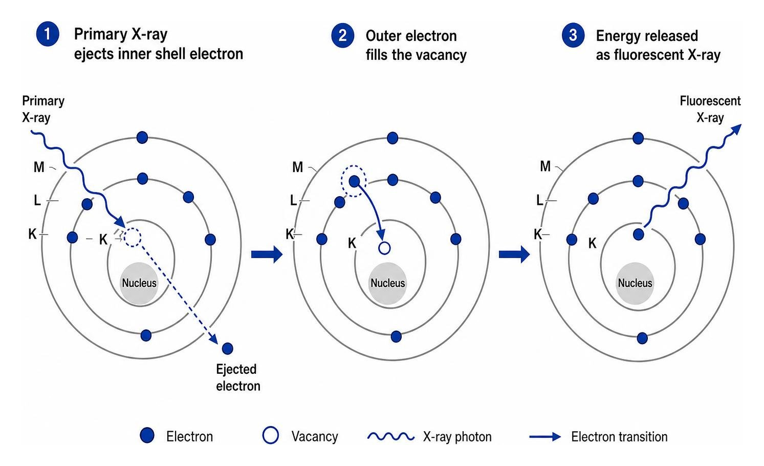
Because the energy difference between any two electron shells is a unique, fixed value for every single element on the periodic table, the emitted X-ray photon has a highly specific energy. By measuring the energy of these emitted secondary X-rays, we can pinpoint exactly which elements are present in the sample. By measuring the intensity (the number of photons detected per second), we can calculate how much of each element is there.

Fundamental Physics of X-Ray Fluorescence

To get a bit more technical, the transitions between electron shells follow strict quantum mechanical rules. The vacancies in the innermost shell (the K shell) are typically filled by electrons from the L shell (producing $K\alpha$ radiation) or the M shell (producing $K\beta$ radiation). Similarly, vacancies in the L shell are filled by outer electrons, producing $L\alpha$ or $L\beta$ spectral lines.

This relationship is governed by Planck’s Law:

$$E = \frac{hc}{\lambda}$$

Where $E$ is the energy of the photon, $h$ is Planck’s constant, $c$ is the speed of light, and $\lambda$ is the wavelength. This means that every characteristic X-ray has both a unique energy and a corresponding unique wavelength.

However, not every ionization event results in the emission of a fluorescent X-ray. Sometimes, the excess energy is transferred to another outer electron, which is then ejected from the atom instead of a photon. This is known as the Auger effect. The probability that an excited atom will emit a fluorescent photon rather than an Auger electron is called the fluorescent yield. The fluorescent yield increases dramatically with atomic number; heavy elements (like lead or gold) are highly efficient fluorescers, whereas light elements (like sodium or carbon) have very low fluorescent yields, making them much harder to detect.

If you are new to these concepts and want a gentle introduction, you can explore our Beginners Guide to X-Ray Fluorescence to build a solid foundation.

Elements Detected and Limits of Detection

In routine laboratory settings, XRF is used to analyze elements from sodium (atomic number $Z = 11$) all the way up to uranium ($Z = 92$). With specialized, ultra-high-performance setups operating under a tight vacuum or helium atmosphere, it is theoretically possible to detect elements as light as beryllium ($Z = 4$).

The detection limits of XRF vary widely depending on the element, the instrument type, and the sample matrix:

• Major Elements: For common bulk geological and industrial elements (such as silicon, titanium, aluminum, iron, manganese, magnesium, calcium, sodium, potassium, and phosphorus), XRF routinely delivers highly accurate measurements in weight percent concentrations.
• Trace Elements: For heavier trace elements (such as barium, cobalt, chromium, copper, nickel, rubidium, strontium, zinc, and zirconium), detection limits in solid samples like rocks and soils are typically on the order of a few parts per million (ppm)—specifically for abundances greater than 1 ppm.
• Light Elements: Because of their low fluorescent yields and low-energy X-rays (which are easily absorbed by the air or the sample itself), elements lighter than sodium are difficult to analyze without comprehensive background and inter-element corrections.

Instrumentation: EDXRF vs. WDXRF Spectrometry

All standard laboratory XRF instruments share a few core components: a primary X-ray source, a sample chamber, and a detection system. The primary beam is typically produced using an X-ray tube with a target material made of rhodium (Rh), though tungsten (W), molybdenum (Mo), or chromium (Cr) targets are also used.

To learn more about the engineering behind these systems, you can refer to classic academic texts like the Encyclopedia of Materials Characterization.

The biggest dividing line in XRF technology is how the instrument separates and measures the emitted secondary X-rays. This splits the market into two distinct categories: Energy-Dispersive (EDXRF) and Wavelength-Dispersive (WDXRF) spectrometry.

Energy-Dispersive X-Ray Fluorescence (EDXRF)

EDXRF spectrometers are the simpler, more compact of the two. In an EDXRF system, the entire fluorescent signal from the sample is directed straight into a solid-state detector—most commonly a Silicon Drift Detector (SDD) or a lithium-drifted silicon [Si(Li)] detector.

The detector measures the energy of each incoming photon directly and converts it into an electrical pulse. Because the detector processes all wavelengths simultaneously, EDXRF is incredibly fast. However, because the detector is hit with a flood of different energies at once, it can suffer from “pulse pile-up”—a phenomenon where successive photons arrive too quickly, overlapping and causing the electronics to miscalculate their energies.

Modern instruments use high-speed digital pulse processors to manage this trade-off between count-rate (speed) and energy resolution, effectively reducing pile-up and baseline shifts. If you want to see how these mechanics are simplified for everyday use, check out our resource X-Ray Fluorescence Spectrometry Explained Simply.

Wavelength-Dispersive Spectrometry (WDXRF)

WDXRF spectrometers are the high-resolution, high-precision giants of the laboratory. Instead of sending the raw fluorescent beam straight to the detector, WDXRF physically separates the X-rays by their wavelengths before they reach the sensor.

It does this using an analyzing crystal. When the divergent fluorescent beam hits this crystal, only X-rays of a very specific wavelength will undergo constructive interference and reflect off the crystal planes at a given angle. This physical sorting is governed by Bragg’s Law:

$$n\lambda = 2d \sin\theta$$

Where $n$ is an integer, $\lambda$ is the wavelength, $d$ is the spacing between crystal planes, and $\theta$ is the angle of incidence. By rotating the analyzing crystal and the detector using a highly precise mechanical device called a goniometer, the instrument can scan through the entire spectrum, measuring one wavelength at a time.

Because WDXRF physically filters out competing wavelengths, it achieves spectacular spectral resolution (often around 24 eV at the manganese peak, compared to 145 eV for a typical EDXRF system). This eliminates peak overlaps and provides incredibly low detection limits.

To help you decide which type of instrument fits your laboratory’s needs, we have compiled an in-depth review of The Best X-Ray Fluorescence Equipment to Upgrade Your Analysis.

Comparing EDXRF and WDXRF

Performance Metric	Energy-Dispersive (EDXRF)	Wavelength-Dispersive (WDXRF)
Spectral Resolution	Moderate (120–150 eV)	Excellent (15–30 eV)
Detection Limits	Good (down to 10–50 ppm)	Superior (down to sub-ppm levels)
Speed of Analysis	Very Fast (simultaneous multi-element)	Slower for sequential scans; fast for simultaneous channels
Portability	High (can be made handheld, < 2 kg)	Low (heavy, benchtop or floor-standing units)
Cost	Budget-friendly to moderate	High to very high
Best Used For	Field screening, alloy sorting, rapid QC	High-precision research, major element geology

Sample Preparation and Overcoming Matrix Effects

One of the biggest myths about XRF is that you can always just throw a raw sample into the machine and get perfect results. While XRF is incredibly versatile, the accuracy of your quantitative data is heavily dependent on how you prepare your sample and how you account for physical and chemical “matrix effects.”

Because secondary X-rays from lighter elements can only escape from the top few micrometers of a sample, the surface of the specimen must be perfectly flat and representative of the bulk material. If the surface is rough or uneven, it will scatter the X-rays unpredictably, violating the strict geometric assumptions of the calibration models. To prevent this, samples are often spun at 5 to 20 rpm during analysis to average out minor surface irregularities.

Furthermore, because air attenuates low-energy X-rays, high-performance analysis of lighter elements (below sodium) requires the sample chamber to be held under a tight vacuum of around 10 Pa. For volatile or liquid samples that would boil or explode in a vacuum, the chamber is instead swept with helium gas.

Common Sample Preparation Methods

Depending on your material and accuracy requirements, we generally use one of several sample preparation pathways:

1. Loose Powders: The fastest method. The sample is ground to a fine powder and poured into a plastic cup sealed with a thin Mylar film. This is excellent for rapid qualitative screening but suffers from particle-size variations and packing density inconsistencies.
2. Pressed Pellets: The powdered sample is mixed with a binder (like wax or cellulose) and pressed under high pressure (typically 20–30 tons) to form a flat, solid disk. This provides much better geometry than loose powder and is widely used for trace element analysis.
3. Glass Fusion Beads: The gold standard for major element analysis in geology and mining. The powdered sample is mixed with a chemical flux (such as lithium tetraborate) and melted in a platinum crucible at temperatures exceeding 1000°C. The molten mixture is poured into a mold to cool into a perfectly homogeneous glass disk. This completely eliminates grain-size discrepancies and mineralogical variations.

For step-by-step instructions and technical checklists on preparing these matrices, you can download our comprehensive guide: Get Glowing With This Complete X-Ray Fluorescence PDF Guide.

Matrix Effects: Absorption and Enhancement

Once the sample is in the machine, we have to deal with the physics of the matrix itself. Matrix effects occur because the atoms in a sample do not exist in a vacuum—they are surrounded by other atoms that can absorb or enhance the fluorescent signal:

• Absorption: The primary or secondary X-rays can be absorbed by other elements in the sample before they can escape. For example, if you are trying to measure silicon in an iron-rich matrix, the heavy iron atoms will absorb a large portion of the weak silicon X-rays, making the silicon concentration appear lower than it actually is.
• Enhancement: The fluorescent X-rays from a heavy element can act as a secondary excitation source for lighter elements. For instance, fluorescent X-rays emitted by nickel atoms have just the right energy to excite iron atoms. If your sample has both, the iron signal will be artificially boosted by the nickel, making the iron concentration appear higher.

To achieve accurate quantitative analysis, we use advanced mathematical models—such as Fundamental Parameters (FP) or empirical calibrations using well-characterized, compositionally similar reference standards—to correct for these inter-element effects.

Practical Applications of XRF in the Field and Lab

XRF’s unique combination of speed, non-destructive nature, and multi-element capabilities has made it indispensable across a vast array of industries. From scanning historical 17th-century paintings to mapping the grade of ore in a deep-earth mining operation, the real-world utility of this technology is incredibly broad.

To see a comprehensive breakdown of where this technology is deployed globally, explore The Ultimate List of Practical XRF Applications.

Environmental Analysis: Soil, Water, and Air

In environmental science, XRF has emerged as a premier tool for supporting green analytical chemistry. Because it requires minimal sample preparation and no hazardous dissolving reagents (like hydrofluoric acid), it allows laboratories to dramatically scale up their testing throughput without generating chemical waste.

• Soil and Geological Testing: XRF is used to map soil contamination, identifying hotspots of heavy metals like lead, arsenic, cadmium, and chromium in industrial brownfields or agricultural land.
• Air Quality Monitoring: Environmental agencies collect air particulate matter (aerosols) on thin membrane filters. XRF can analyze these filters directly, measuring the concentrations of sulfur, lead, and other airborne elements to track pollution sources.
• Vegetation and Agriculture: Researchers use XRF to study trace element uptake in crops and native vegetation, helping to optimize fertilizers and monitor environmental health.
• Water and Aqueous Extracts: While liquid water is a challenging matrix for XRF due to its light-element composition, target elements can be pre-concentrated onto membrane filters or analyzed via specialized total reflection X-ray fluorescence (TXRF) setups.

Handheld XRF and Field Analysis

The development of miniature, low-power X-ray tubes and high-resolution silicon drift detectors has revolutionized field analysis. Today, portable handheld XRF analyzers weigh less than 2 kg yet pack the analytical power that once required a room-sized instrument.

These devices are widely used for:

• Scrap Metal Sorting: Instantly identifying alloy grades (such as distinguishing 304 from 316 stainless steel) in recycling yards.
• Consumer Product Safety: Screening imported toys and plastics for restricted hazardous substances under RoHS regulations.
• Residential Safety: Testing painted surfaces for lead content. For parents worried about older homes, we have put together a detailed walkthrough: XRF Lead Based Paint Testing Explained for Concerned Parents.

Strengths, Limitations, and Alternative Techniques

While we love XRF for its speed and versatility, no single analytical tool is perfect. To choose the right method for your project, you must weigh its strengths against its inherent physical boundaries.

Strengths of XRF:

• Non-Destructive (Mostly): Solid samples (like metals, coins, or art) can be analyzed without leaving a scratch. (Note: glass fusion and pressed pellet preparation are physically destructive to the original sample structure, but the chemical sample remains preserved in the disk).
• Extremely Fast: Qualitative screening results are available in seconds; high-precision quantitative runs take only minutes.
• Cost-Effective: Low operating costs per sample because it requires no consumable gases or chemical reagents.
• Broad Elemental Range: Covers almost the entire periodic table in a single run.

Limitations of XRF:

• No Valence State Information: XRF cannot tell you the oxidation state of an element. It will tell you the total iron content, but not whether it is $Fe^{2+}$ or $Fe^{3+}$. For valence states, you must use wet chemistry or Mössbauer spectroscopy.
• No Isotopic Information: XRF cannot distinguish between different isotopes of the same element (e.g., Lead-206 vs. Lead-208). This requires mass spectrometry techniques like ICP-MS.
• Light Element Sensitivity: Quantifying elements lighter than sodium remains difficult and prone to high measurement uncertainty.
• Bulk Analysis Only: Standard XRF analyzes a relatively large bulk area (typically 10–40 mm in diameter) rather than micron-scale spots, though modern micro-XRF units are beginning to bridge this gap.

If your project requires trace element sensitivity beyond the limits of standard XRF, or if you need to analyze exceptionally thin surface layers, you should consider alternative ion-beam techniques. To learn more, read our deep-dive: The Ultimate Guide to Particle Induced X-Ray Emission.

XRF vs. PIXE (Proton Induced X-Ray Emission)

At Elemental Analysis Inc., we are proud to operate the first commercial PIXE laboratory. While both XRF and PIXE rely on the emission of characteristic secondary X-rays to identify elements, they differ fundamentally in how they excite the atoms.

Where XRF uses a beam of X-ray photons, PIXE uses a focused beam of high-energy protons produced by a particle accelerator. This difference yields several key analytical advantages:

• Background Noise: Protons produce far less background Bremsstrahlung radiation than X-ray photons. This results in a much higher signal-to-noise ratio.
• Sensitivity: Because of the lower background noise, PIXE can achieve detection limits in the sub-ppm range for many trace elements—often a full order of magnitude more sensitive than standard EDXRF.
• Micro-Analysis: Proton beams can be focused down to sub-micrometer spot sizes, allowing for high-resolution elemental mapping of highly heterogeneous samples.

To see if this advanced ion-beam technique is the right fit for your analytical challenges, explore our dedicated page on PIXE.

Recent Trends and Quality Assurance in XRF

The world of X-ray spectrometry is moving fast. Recent literature reviews, such as the 2023 atomic spectrometry update, highlight several exciting technological leaps that are reshaping the industry:

1. Synchrotron Radiation XRF (SR-XRF): By utilizing massive particle accelerators as X-ray sources, researchers are achieving nanometer-scale spatial resolution with limits of detection pushed down to the parts-per-billion (ppb) level.
2. MacroXRF and Machine Learning: In cultural heritage and art conservation, macroXRF scanners are used to map entire paintings, revealing hidden layers and past restorations. Because these scans produce massive datasets, scientists are deploying machine-learning algorithms to automatically process and classify the elemental maps.
3. Total Reflection XRF (TXRF) in Biomedicine: TXRF is seeing a steep rise in biomedical applications, allowing researchers to analyze minute tissue samples (as small as 20 mg) of blood, placenta, or heart tissue with extreme precision.

Quality Assurance and Calibration Practices

No matter how advanced the instrument is, the data is only as good as the quality assurance (QA) practices behind it. To ensure our clients receive rock-solid, legally defensible data, we adhere to strict QA/QC protocols:

• Reference Materials: We regularly run certified reference materials (CRMs)—well-characterized standards of known composition—alongside client samples to verify accuracy.
• Drift Correction: X-ray tubes and detectors age over time, which can cause minor shifts in signal intensity. We use specialized drift correction standards to recalibrate the instrument’s intensity scale automatically.
• Blank Monitoring: Running blank samples ensures that no cross-contamination has occurred during the sample preparation process (such as contamination from grinding plates).

Frequently Asked Questions about XRF

What is the difference between EDXRF and WDXRF?

The primary difference lies in how they sort the emitted X-rays. EDXRF measures the energy of all incoming X-rays simultaneously using a solid-state detector, making it fast, compact, and ideal for portable field applications. WDXRF uses an analyzing crystal to physically diffract and separate the X-rays by wavelength before they hit the detector. This delivers much higher spectral resolution and lower detection limits, but requires a larger, more expensive, and less portable laboratory instrument.

What elements cannot be detected by XRF?

Standard commercial XRF instruments cannot routinely detect the lightest elements on the periodic table: hydrogen, helium, and lithium. These elements have extremely low fluorescent yields, and their characteristic X-rays are so weak that they are entirely absorbed by the sample itself or the detector’s window before they can be measured.

Is XRF completely non-destructive?

For solid, stable objects like metal alloys, coins, or historical artifacts, XRF is 100% non-destructive; the sample is completely unaltered by the analysis. However, for geological, environmental, or ceramic samples, achieving high-precision quantitative results requires grinding the sample into a fine powder to press into a pellet or melt into a glass fusion bead. In these cases, the physical structure of the original sample is destroyed, though its chemical components remain entirely preserved in the prepared disk.

Conclusion

Whether you need to screen soil for heavy metals, verify the alloy composition of an aerospace component, or conduct high-precision geological research, X-ray fluorescence offers an elegant, non-destructive, and green analytical solution.

At Elemental Analysis Inc., based in Lexington, Kentucky, we combine decades of analytical expertise with a suite of cutting-edge testing capabilities. As the pioneers of the first commercial PIXE laboratory, we understand the physics of X-rays inside and out. We are dedicated to providing our clients with rapid turnarounds, competitive pricing, and highly accurate elemental identification and quantification.

Ready to take your material characterization to the next level? Contact us today to discuss your project, or explore our specialized XRF Services to find the perfect analytical path for your needs.