X-Ray Fluorescence Spectrometry Explained Simply

What X-Ray Fluorescence Spectrometry Actually Is (And Why It Matters)

X-ray fluorescence spectrometry is a non-destructive analytical technique that identifies and measures the elemental composition of a material by exposing it to high-energy X-rays and measuring the characteristic secondary X-rays it emits in response.

Here is a quick summary of what you need to know:

• What it does: Tells you which elements are present in a sample and how much of each is there
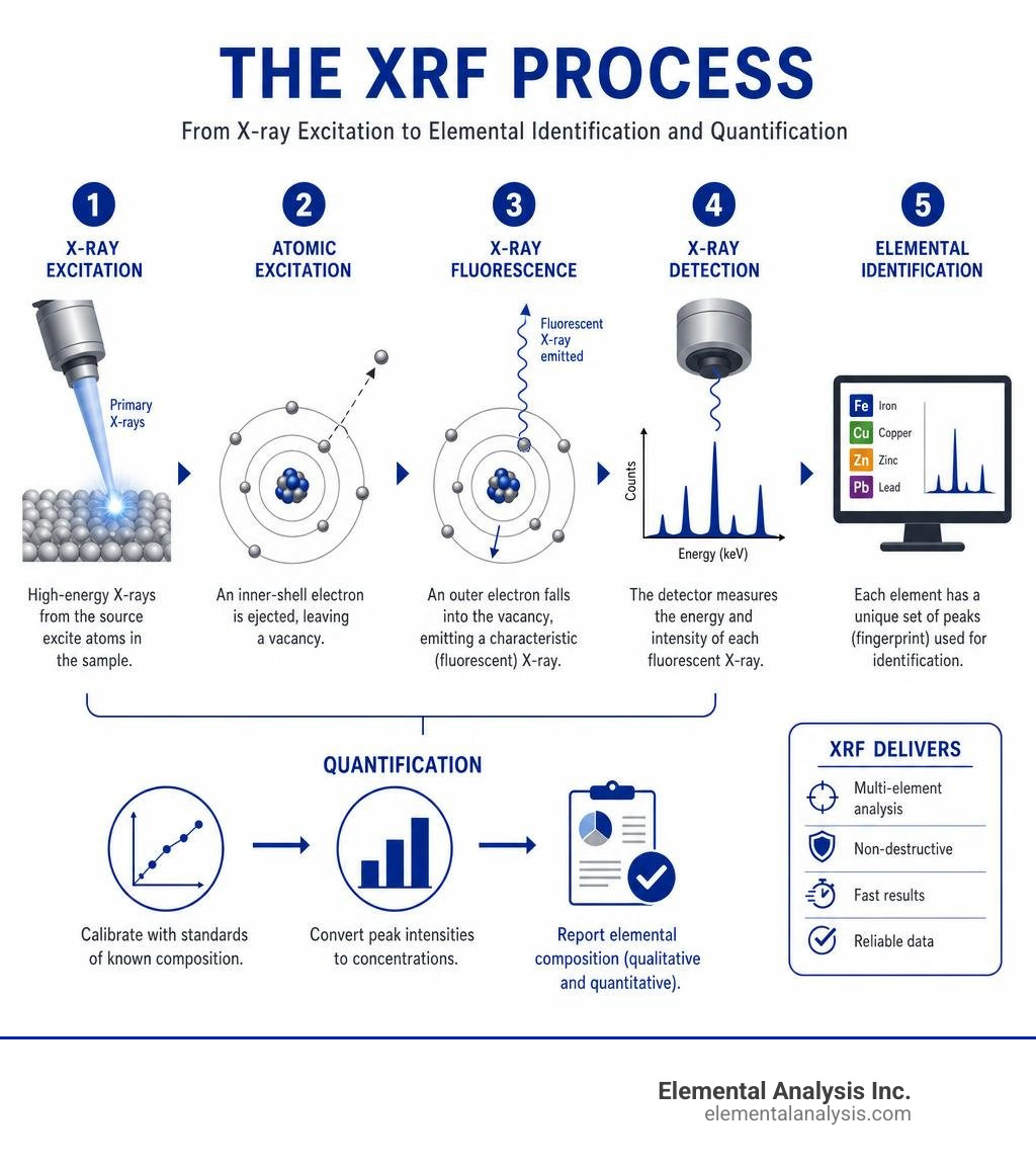
• How it works: A primary X-ray beam excites atoms in the sample; those atoms release characteristic fluorescent X-rays that act as a unique elemental fingerprint
• What it can measure: Elements from sodium (Z=11) up to uranium routinely; concentrations from sub-ppm trace levels all the way up to 100%
• Sample types: Solids, powders, liquids, thin films, filters — often with little or no preparation
• Key advantage: Fast, non-destructive, and capable of multi-element analysis in a single measurement

XRF has been in use since the 1950s and is now one of the most widely relied-upon tools in labs across environmental testing, mining, metals, pharmaceuticals, forensics, and aerospace. Modern instruments — including field-portable units weighing under 2 kg — make it practical both on the bench and in the field.

For lab managers who need fast turnaround, low detection limits, and minimal sample destruction, XRF is often the first technique worth reaching for.

The Core Principles of X-Ray Fluorescence Spectrometry

At its heart, x-ray fluorescence spectrometry relies on a simple, elegant physical phenomenon: when you shine high-energy “primary” radiation onto an atom, the atom shines back with its own “secondary” (or fluorescent) radiation.

X-rays sit on the high-energy end of the electromagnetic spectrum, with wavelengths typically ranging from 0.01 to 10 nanometers. Because these wavelengths are so short and their energy is so high, they do not just bounce off the surface of a material; they penetrate into the electronic structure of the atoms themselves.

What makes this technique incredibly valuable is that it is fundamentally non-invasive. Unlike other methods that require you to dissolve your precious sample in boiling acid, XRF leaves the chemical bonds and physical structure of your sample largely intact. If you want to dive deeper into the basics before we get into the heavy physics, check out our Get Glowing with This Complete X-Ray Fluorescence PDF Guide.

How X-Ray Fluorescence Spectrometry Works at the Atomic Level

To understand how this works, we need to take a quick trip back to high school chemistry. Imagine an atom as a tiny solar system. The nucleus is at the center, surrounded by electrons orbiting in specific “shells” or energy levels. The shell closest to the nucleus is the K shell, followed by the L shell, the M shell, and so on.

Here is the step-by-step atomic dance that occurs during XRF:

1. Excitation: A high-energy primary X-ray photon strikes an atom in the sample. If this photon has more energy than the binding energy of an electron in the inner K or L shell, it knocks that electron clean out of its orbit.
2. The Vacancy: This leaves the atom in an unstable, highly excited state. It now has a “hole” or vacancy in its inner shell.
3. The Transition: To restore stability, an electron from a higher-energy outer shell (like the L or M shell) immediately drops down to fill the vacancy.
4. Fluorescence Emission: Because the outer shell electron has more energy than the inner shell vacancy requires, it must shed its excess energy. It does this by releasing a single photon of secondary radiation—this is the fluorescent X-ray.

Because the energy spacing between electron shells is highly specific to each element, the emitted photon has an exact, characteristic energy. For example, when an electron drops from the L shell to the K shell, it emits what we call a $K\alpha$ X-ray. If it drops from the M shell to the K shell, it emits a $K\beta$ X-ray.

This relationship is governed by Moseley’s Law, which proves that the square root of the frequency of the emitted X-ray is directly proportional to the atomic number ($Z$) of the element. In plain English: the heavier the element, the higher the energy of its fluorescent X-rays. This energy acts as a unique atomic fingerprint. Learn more about the physics of X-ray fluorescence to see how these transitions map across the periodic table.

However, not every excited atom successfully emits a fluorescent photon. Sometimes, the excess energy is transferred to another outer electron, ejecting it instead—a process known as the Auger effect. The probability of an atom emitting a fluorescent photon instead of an Auger electron is called the “fluorescence yield.” This yield drops off sharply for lighter elements, which is why detecting elements lighter than sodium (Z=11) is notoriously tricky.

Instrumentation and Detection in X-Ray Fluorescence Spectrometry

How do we turn these atomic transitions into readable data? A standard XRF spectrometer consists of three primary components: the excitation source, the sample chamber, and the detection system.

• The Excitation Source: In most laboratory instruments, this is an X-ray tube. These tubes typically operate in the 20 to 60 kV range, firing a stream of electrons at a target material (such as rhodium, tungsten, molybdenum, or chromium) to generate a high-intensity primary X-ray beam. Some portable devices use radioisotope sources instead, while high-end research facilities use synchrotron radiation for ultra-high flux.
• The Detector: The detector’s job is to capture the emitted fluorescent photons and measure either their energy or their wavelength. Modern systems primarily use silicon drift detectors (SDDs) or older lithium-drifted silicon [Si(Li)] detectors, which are cooled via Peltier elements or liquid nitrogen. For specific wavelengths, gas proportional counters or scintillation counters are used.
• The Atmosphere: Because air absorbs low-energy X-rays, analyzing light elements requires managing the sample environment. Instruments will pull a vacuum (often down to around 10 Pa) or use a helium purge to ensure those weak, light-element signals actually make it to the detector instead of getting lost in the air.

The detector converts the incoming X-ray photons into electrical pulses. A pulse processor then sorts these pulses by height (which corresponds to photon energy), building up a spectrum where the position of the peaks identifies the elements, and the height of the peaks tells us how much of each element is present. For an in-depth look at how these components are engineered, take a look at this Technical guide on XRF instrumentation.

Comparing EDXRF vs. WDXRF Spectrometers

If you are looking to bring XRF capability into your workflow, you will quickly find that the market is split into two major camps: Energy-Dispersive (EDXRF) and Wavelength-Dispersive (WDXRF) spectrometers.

The fundamental difference lies in how they separate and measure the incoming fluorescent X-rays:

Feature	Energy-Dispersive (EDXRF)	Wavelength-Dispersive (WDXRF)
Separation Method	Electronic sorting via solid-state detector	Physical diffraction using monochromator crystals
Spectral Resolution	150 to 300 eV (broader peaks)	5 to 20 eV (extremely sharp peaks)
Element Range	Sodium (Na) to Uranium (U)	Beryllium (Be) to Uranium (U)
Analysis Speed	Fast (simultaneous multi-element)	Can be slower (sequential) or very fast (simultaneous multi-channel)
Portability	High (handheld units weigh < 2 kg)	Low (typically large, benchtop or floor-standing)
Cost	Budget-friendly to moderate	High capital investment

Choosing between these two technologies depends heavily on your laboratory’s throughput requirements, budget, and the specific elements you need to measure. If you are weighing your options, our guide on The Best X-Ray Fluorescence Equipment to Upgrade Your Analysis offers a detailed breakdown of the top instruments available in 2026.

Energy-Dispersive XRF (EDXRF)

EDXRF instruments are the workhorses of rapid screening. In an EDXRF system, the entire fluorescent signal from the sample is directed straight into a solid-state detector. The detector and its associated electronics sort the incoming photons by energy on the fly.

Because there are no moving optical parts, EDXRF systems are mechanically simple, robust, and highly compact. This simplicity makes them ideal for portable and handheld devices. Modern handheld EDXRF “guns” are incredibly convenient, utilizing Peltier-cooled silicon detectors that don’t require bulky liquid nitrogen. They allow field operators to point, shoot, and get a multi-element analysis of alloys, soils, or consumer goods in a matter of seconds.

Wavelength-Dispersive XRF (WDXRF)

WDXRF systems are the gold standard for high-precision laboratory analysis. Instead of sending the whole messy signal to the detector at once, WDXRF uses physical crystal monochromators to separate the X-rays by wavelength before they reach the detector.

This separation relies on Bragg’s Law:

$$n\lambda = 2d\sin\theta$$

By rotating an analyzing crystal (with a known atomic spacing, $d$) and the detector relative to the sample using a high-precision goniometer, the system selects specific wavelengths ($\lambda$) to measure one by one.

Because the physical separation of wavelengths yields incredibly sharp peaks (resolutions of 5–20 eV compared to EDXRF’s 150–300 eV), WDXRF virtually eliminates spectral overlaps. This makes it unmatched for trace element analysis and for measuring light elements down to beryllium. Simultaneous WDXRF systems equipped with multiple fixed-channel detectors can even complete high-precision analyses of up to 30 elements in under 30 seconds, making them indispensable for quality control in cement and metallurgical plants.

Key Applications of XRF in Environmental Analysis

In recent years, the analytical community has embraced “green analytical chemistry” (GAC). The goal of GAC is simple: minimize chemical waste, reduce the use of hazardous reagents, and simplify sample preparation. Because XRF is a solid-state, non-destructive technique, it fits perfectly into this green philosophy.

Environmental scientists routinely use XRF to monitor soils, air quality, water, vegetation, and industrial waste. For a broader look at how this technology is used across other sectors, check out The Ultimate List of Practical XRF Applications.

Soil and Geological Mapping

When it comes to assessing contaminated sites or mapping geological formations, XRF is a game-changer. Historically, analyzing soil for heavy metals meant collecting samples, driving them back to a lab, digesting them in hot acid, and running them through an ICP-OES.

With field-portable EDXRF analyzers, environmental engineers can get real-time data directly on-site. These lightweight devices can screen for hazardous metals like lead, arsenic, and chromium in seconds. For example, modern handheld units can achieve limits of detection around 2 parts per million (ppm) of lead in pure sand.

In mining exploration, geologists use portable XRF for geochemical mapping, allowing them to rapidly identify ore boundaries and make immediate decisions on where to drill next.

Air Particulates and Aerosols

Monitoring the air we breathe requires collecting airborne particulate matter (such as PM2.5 and PM10) on thin membrane filters (such as Teflon or Nuclepore). Because these sample masses are incredibly small—often just a few micrograms of dust spread across a filter—traditional wet chemical analysis is extremely difficult.

XRF is uniquely suited for this. Because the sample is presented as a thin film, there is very little matrix absorption of the X-rays. Standardized protocols, such as the EPA Compendium Method IO-3.3 for air particulates, outline how to use energy-dispersive XRF to non-destructively determine up to 44 elements on a single filter.

To prevent damaging the delicate filters, these systems often use “secondary excitation.” Instead of hitting the filter directly with the raw X-ray tube beam, the beam is directed at a secondary target (like a metal foil), which fluoresces and sends a gentler, monochromatic beam to the sample.

Water, Vegetation, and Waste Monitoring

While XRF is traditionally a solid-sample technique, advances in sample preparation have expanded its reach to liquids and organic tissues:

• Aqueous Extracts and Waters: Direct liquid analysis in XRF is possible using specialized sample cups with thin Mylar bottoms. However, for trace analysis, scientists often use Total Reflection X-Ray Fluorescence (TXRF). By evaporating a tiny droplet of water (as small as 20 microliters) onto a polished quartz carrier, the X-ray beam hits the sample at a grazing angle, minimizing background scatter and pushing detection limits down to the parts-per-billion (ppb) level.
• Vegetation: Analyzing plant tissues for nutrient uptake or heavy metal accumulation typically involves drying, grinding, and pressing the leaves into pellets. This fast, chemical-free prep aligns perfectly with green chemistry goals.
• Waste Monitoring: XRF is used to screen municipal and industrial waste for hazardous materials before disposal, ensuring compliance with environmental regulations and identifying recyclable metals in electronic scrap.

Qualitative vs. Quantitative Analysis: Accuracy and Detection Limits

XRF is highly versatile; it can be used for both quick qualitative screening and highly accurate quantitative testing.

• Qualitative Analysis: This is the “what is in there?” phase. Because peak energy corresponds directly to a specific element, identifying elements is as simple as finding where the peaks land on the energy scale of the spectrum.
• Quantitative Analysis: This is the “how much is in there?” phase. In theory, peak intensity (the area under the peak) is proportional to the concentration of the element. In practice, it is rarely that simple due to matrix effects.

Matrix effects occur because the other elements in the sample can absorb or enhance the fluorescent X-rays of the target element. For instance, if you are measuring iron in a sample that also contains a lot of nickel, the nickel atoms will absorb the iron X-rays and re-emit their own, artificially lowering your iron reading.

To correct for these interferences, scientists use two main calibration approaches:

1. Empirical Calibration: This method uses Certified Reference Materials (CRMs) that are physically and chemically similar to the unknown samples. By plotting a calibration curve of known concentration versus peak intensity, the instrument can calculate the unknown concentrations.
2. Fundamental Parameters (FP): This is a standardless mathematical approach. It uses physics-based equations (accounting for X-ray tube output, absorption coefficients, and detector efficiency) to calculate concentrations. FP is incredibly useful when you do not have a matching standard for a unique sample.

To keep up with the latest software and calibration advances, you can read the 2023 atomic spectrometry update on XRF advances, which highlights how machine learning is now being integrated to automate spectrum deconvolution and matrix corrections.

Safety Considerations and Regulatory Requirements

Because XRF instruments generate ionizing radiation, safety is a top priority. However, there is no need to panic—modern instruments are engineered with multiple layers of protection.

Laboratory benchtop and floor-standing XRF systems feature fully shielded, closed sample cabinets. These cabinets include safety interlocks that physically prevent the X-ray tube from firing if the door is open. When operated correctly, these systems expose users to virtually zero radiation.

Handheld and portable XRF devices require more active operator safety because they have an open beam path. When using a handheld device, operators must adhere to the ALARA (As Low As Reasonably Achievable) principle:

• Time: Minimize the time spent near an active beam.
• Distance: Keep your hands and body away from the front of the analyzer. Never point the device at yourself or anyone else.
• Shielding: Use backscatter shields when testing low-density materials (like plastics or thin alloys) that allow X-rays to pass through and scatter back toward the user.

In most jurisdictions, registering your XRF instrument with local radiation safety authorities is required. Operators must undergo formal radiation safety training, and facilities often appoint a Radiation Safety Officer (RSO) to manage compliance, perform routine leak testing, and monitor personal dosimetry badges.

Frequently Asked Questions about XRF

What is the lightest element XRF can detect?

In theory, WDXRF systems can detect elements as light as beryllium ($Z=4$). However, in practical, routine laboratory settings, sodium ($Z=11$) or fluorine ($Z=9$) is the typical cutoff. Light elements have very low fluorescence yields and emit ultra-low-energy X-rays that are easily absorbed by the sample itself, the air, or the detector window.

Is XRF analysis completely non-destructive?

For many samples, yes. If you place a metal alloy, a coin, or a plastic part into the chamber, it will come out completely unchanged. However, for geological and powder samples, achieving high accuracy requires grinding the sample into a fine powder and pressing it into a pellet or fusing it with a borate flux into a glass bead. While the material is not chemically destroyed, its original physical form is altered.

How does XRF compare to ICP-MS?

Inductively Coupled Plasma Mass Spectrometry (ICP-MS) offers vastly superior detection limits (often down to parts-per-trillion) and can measure lighter elements and isotopes. However, ICP-MS requires completely dissolving the sample in strong acids, destroying it in the process. XRF is much faster, requires virtually no sample preparation, is completely solid-state, and is far more cost-effective for major and trace element screening.

Conclusion

X-ray fluorescence spectrometry is a cornerstone of modern analytical chemistry. Its balance of speed, non-destructive testing, and multi-element capability makes it an indispensable tool for environmental monitoring, industrial quality control, and scientific research.

At Elemental Analysis Inc., located in Lexington, Kentucky, we understand that choosing the right analytical path can be daunting. As the first commercial PIXE (Proton-Induced X-ray Emission) laboratory, we specialize in high-accuracy trace element identification, quantification, and speciation. Whether you need the rapid screening of XRF or the ultra-trace capabilities of our specialized nuclear and chemical techniques, our team is dedicated to providing fast turnaround and highly competitive pricing.

Ready to see what is hidden inside your materials? Explore our XRF services today, or get in touch with our Lexington-based experts to find the perfect testing solution for your industry.